This guide outlines the design and implementation of A networks for AI Modeling training clusters. The focus is on providing a lossless, high-throughput, and low-latency network that meets the demands of large-scale AI models. This document goes into detail about architecture, configurations, and key features such as RoCEv2 and intelligent lossless networking.
1. Overview of AI and Deep Learning
1.1 Artificial Intelligence Concepts
Artificial Intelligence (AI) is the simulation of human intelligence processes by machines, particularly computer systems. It includes:
- Narrow AI (Weak AI): Designed to perform specific tasks (e.g., Siri, AlphaGo).
- General AI (Strong AI): Can theoretically handle any intellectual task that humans can.
- Super AI: Hypothetical AI that surpasses human intelligence across all domains (not yet realized).
1.2 Deep Learning and Distributed Training
Deep Learning (DL) is a subset of AI that simulates human neural networks. These networks are composed of multiple layers (deep networks), making them ideal for tasks such as image recognition, NLP, and autonomous decision-making. Deep learning models typically require distributed training across multiple servers due to their computational intensity.
Deep Learning Workflow:
- Data Collection: Massive datasets from various sources are processed.
- Model Training: Neural networks are trained on distributed GPUs or TPUs, requiring significant computational resources.
- Parameter Exchange: Gradients are shared across nodes during each training iteration.
- Model Evaluation: The trained model is deployed for inference, making predictions on new data.
Distributed Training Communication
In distributed training, data needs to be efficiently transferred between nodes during training processes. A few key components are:
- Forward Propagation (FP): Input data passes through the layers of the neural network.
- Backward Propagation (BP): Gradients are calculated and shared back to adjust the model’s parameters.
- Allreduce Operation: A communication operation used to sum or average gradients across multiple nodes, ensuring that model parameters are synchronized.
Key Training Communication Models:
- Ring-Allreduce: Organizes nodes into a ring, reducing communication complexity and improving speed.
- Halving-Doubling: Reduces computational load by splitting the data, improving efficiency for large-scale AI tasks.
2. Intelligent Lossless Network Overview
2.1 What is an Intelligent Lossless Network?
An intelligent lossless network ensures zero packet loss, maximum throughput, and low latency, which are crucial for high-performance AI and HPC environments. These networks rely on RoCEv2 (RDMA over Converged Ethernet) to minimize CPU overhead and allow direct memory access between nodes, significantly improving the efficiency of distributed AI training.
2.2 Key Features
- Zero Packet Loss: Essential for AI workloads where packet loss can cause major delays in model training.
- High Throughput: Supports massive data transfers, ensuring that all GPUs or NPUs are fully utilized during the training process.
- Low Latency: Critical for real-time AI applications like robotics or autonomous systems.
- RoCEv2 Support: Provides RDMA over Ethernet, reducing CPU overhead and accelerating memory access.
3. AI Scenario Network Design
3.1 Overall Network Architecture
The AI training network is divided into multiple segments based on functionality:
- Access Zone: Manages external internet connections and dedicated lines.
- Management Zone: Responsible for the management of servers, storage, and networking devices.
- AI Cluster Zone: The primary zone for AI training, where compute nodes process data.
- Storage Zone: Dedicated to high-speed, high-bandwidth access to distributed storage systems for training datasets, checkpoints, and logs.
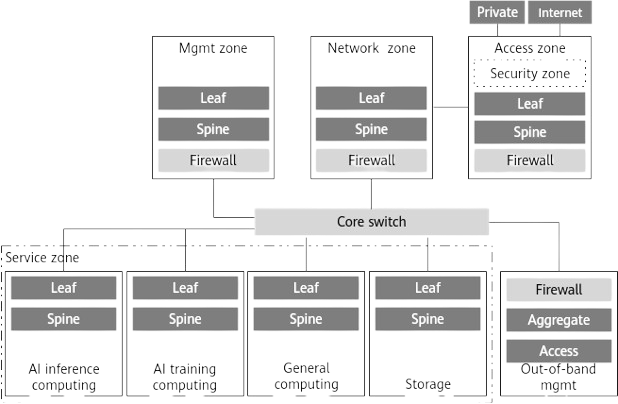
Figure: AI Network Logical Architecture
This figure shows the AI network’s logical structure, with each zone clearly defined and connected via core switches.
3.2 Physical Network Design (Underlay)
The physical layer is based on a two-tier CLOS (Spine-Leaf) architecture designed to provide high bandwidth and low latency, accommodating the immense data transfer needs of large-scale AI training.
3.2.1 Two-Tier CLOS Architecture
Figure: Two-Tier Spine-Leaf Architecture
The Spine-Leaf architecture connects every server and storage system through high-speed links.
- Spine Layer: Consists of high-capacity switches that aggregate traffic from the leaf layer.
- Leaf Layer: Connects directly to the servers and storage systems, using high-speed links (100G/400G) to ensure no bandwidth bottlenecks.
- Non-Blocking Architecture: This structure ensures no oversubscription, providing 1:1 bandwidth allocation between Leaf and Spine switches.
- Low Latency: The flat design minimizes the number of hops between nodes, reducing latency to an absolute minimum.
3.3 AI Training Server Access Design
Access to AI servers must be designed to support redundancy, high bandwidth, and fault tolerance. Two main designs are commonly used:
3.3.1 Single-Rail vs. Multi-Rail Access
- Single-Rail Access: Each GPU/NPU card has an independent network interface with a unique IP. This approach avoids link aggregation.
- Advantages: Simple network configuration, easier troubleshooting.
- Drawback: No redundancy in case of link failure.
- Multi-Rail Access: Each AI server is connected to multiple Leaf switches, distributing its GPU/NPU cards across multiple network paths.
- Advantages: Higher redundancy and fault tolerance, balanced load.
- Drawback: Slightly more complex to manage and deploy.
Figure: Server Access Design
This figure compares single-rail and multi-rail access designs, detailing their impact on fault tolerance, redundancy, and performance.
Table: Access Design Comparison
| Criteria | Single-Rail Access (Recommended) | Multi-Rail Access (Supported) |
|---|---|---|
| Fault Tolerance | 4 servers affected per switch | 32 servers affected per switch |
| Deployment Complexity | Easier to deploy copper cables | Requires optical modules |
| Performance | More load on Spine | Load balanced across Spines |
3.4 Logical Network Design (Overlay)
3.4.1 Traditional Non-Cloud Design (L3 Spine-Leaf)
For environments that do not use cloud platforms, the parameter plane network can operate in L3 mode with distributed gateways:
- L3 Leaf-Spine Network: Each Leaf switch handles local routing, while Spine switches manage inter-leaf traffic.
Figure: L3 Network Design for Traditional Environments
3.4.2 Cloud Multi-Tenant Design (VXLAN)
In multi-tenant cloud environments, VXLAN is used to provide Layer 2 overlay networking over a Layer 3 infrastructure, allowing tenants to have isolated virtual networks.
- EVPN-VXLAN: Ensures tenant isolation by providing Layer 2 connectivity across different physical switches, supporting resource pooling and scalability.
Figure: VXLAN Architecture for Multi-Tenant Isolation
This figure shows how VXLAN is deployed in a cloud environment, providing isolated virtual networks for different tenants.
4. Reliability Design
4.1 Single-Link Access
For AI training environments, single-link access is used to connect servers directly to Leaf switches. This approach assumes that fault tolerance is managed by the application itself, through checkpointing and failure recovery mechanisms.
Figure: Single-Link Access Design
Shows the network structure where AI servers connect directly to the network with no link aggregation.
4.2 Multi-Link Access
For higher fault tolerance, multi-link access connects AI servers to multiple Leaf switches. In case of a link or switch failure, traffic is seamlessly redirected through the remaining links.
- Redundancy: If one link fails, the system continues functioning without interruption by rerouting traffic through active links.
- Load Balancing: Multiple links also allow for better load balancing, ensuring the network does not become congested.
Figure: Multi-Link Access Design
Illustrates a high-redundancy setup with multiple network paths between servers and switches.
5. AI Cluster Networking
5.1 AI Sample Plane Design
The sample plane handles high-frequency access to storage for training datasets. It uses a two-tier CLOS design similar to the parameter plane but focuses on high throughput and low latency for large-scale data transfers.
5.1.1 Sample Plane Physical Network
Figure: Sample Plane Network Design
This diagram illustrates the physical layout of the AI sample plane, showing how compute nodes and storage systems are connected via RoCEv2 links to minimize latency.
6. Intelligent Lossless Network Features
6.1 PFC and ECN Configuration
The intelligent lossless network ensures that packet loss is avoided using PFC (Priority Flow Control) and ECN (Explicit Congestion Notification). These protocols manage congestion by adjusting the flow of traffic across the network.
- PFC: Manages priority-based flow control, ensuring no packet loss occurs in critical data streams like RoCEv2.
- ECN: Detects congestion early and adjusts traffic rates to avoid packet loss.
Figure: PFC and ECN Deployment in VXLAN Networks
6.2 Dynamic Load Balancing
AI models generate heavy and periodic data flows. Traditional load balancing based on flow hashing may lead to imbalances. Instead, **NSLB (NetworkScale Load Balancing)** dynamically adjusts traffic distribution across the network, preventing congestion and improving overall performance.
6.2.1 Static vs. Dynamic NSLB
Static NSLB distributes traffic based on fixed rules, ensuring that all paths are used equally under normal conditions. However, Dynamic NSLB-CP (Control Plane) uses real-time data from the AI job scheduler to adjust routing based on current network traffic, optimizing for both fault tolerance and performance.
Figure: Static vs. Dynamic NSLB Comparison
This figure shows the differences between static and dynamic NSLB, highlighting how dynamic load balancing optimizes network throughput and reduces latency in real-time scenarios.
Table: Static vs. Dynamic NSLB
| Feature | Static NSLB | Dynamic NSLB-CP |
|---|---|---|
| Traffic Distribution | Fixed rules | Real-time adjustment |
| Optimal Use of Resources | Medium | High |
| Fault Tolerance | Limited to predefined paths | Dynamically adjusts to failures |
7. Network Monitoring and Telemetry
7.1 Telemetry
Real-time telemetry is essential for ensuring the network runs efficiently. Telemetry enables continuous monitoring of network performance, collecting metrics such as packet loss, congestion events, and bandwidth utilization from network devices.
- Telemetry Data Collection: Switches continuously push metrics to a centralized monitoring system. This allows network administrators to observe trends, identify bottlenecks, and troubleshoot problems before they impact AI workloads.
- Telemetry Granularity: Provides insights at the queue level, monitoring congestion points and helping to fine-tune ECN and PFC settings.
Figure: Telemetry vs. Traditional SNMP Monitoring
This figure compares telemetry-based monitoring with traditional SNMP-based systems, showing how telemetry provides faster, more detailed data for real-time network adjustments.
8. AI Fabric – RoCEv2 and ECN Features
8.1 RoCEv2 (RDMA over Converged Ethernet)
RoCEv2 is critical for ensuring high-performance, low-latency communication between nodes in distributed AI clusters. It leverages RDMA to bypass CPU involvement in data transfer, allowing direct memory access between servers, reducing latency, and increasing throughput.
Key Features of RoCEv2:
- Low Latency: RDMA ensures that data is transferred without CPU intervention, reducing transmission delays.
- Zero Packet Loss: RoCEv2 works with PFC to ensure that packet loss is minimized, which is essential for distributed AI training.
8.2 ECN (Explicit Congestion Notification)
ECN plays a crucial role in congestion control. When network devices detect congestion, ECN marks packets instead of dropping them. This marking triggers a rate adjustment at the source, preventing packet loss while maintaining throughput.
ECN Workflow:
- Congestion Detection: The switch detects congestion based on queue depth.
- Marking Packets: ECN marks the IP header of packets to indicate congestion.
- Rate Adjustment: The receiver informs the sender to reduce the sending rate, preventing further congestion.
Figure: ECN Packet Flow in a RoCEv2 Environment
This diagram demonstrates how ECN manages congestion in a RoCEv2 network by marking packets and adjusting traffic flow.
9. Operational Design and Monitoring
9.1 Network Health Monitoring
To ensure continuous performance, the network requires comprehensive monitoring to detect and prevent issues such as packet loss, link failures, and congestion. Tools like iMaster NCE-FabricInsight provide end-to-end visibility of network performance.
- Health Monitoring Metrics: Monitors metrics such as queue lengths, packet drops, and latency across the entire network. It provides alerts when thresholds are crossed, allowing for proactive management.
- Issue Detection: FabricInsight can identify suboptimal performance issues, like microbursts or buffer overruns, that may not cause complete failures but still degrade AI training efficiency.
Figure: Network Health Monitoring Interface
This figure shows the iMaster NCE-FabricInsight interface, illustrating how network administrators can visualize health metrics and identify potential performance issues in real-time.
10. Design for Scalability and Future Growth
10.1 Scalability in AI Networks
As AI workloads grow, networks must be scalable without requiring major architectural changes. The two-tier Spine-Leaf architecture is inherently scalable:
- Horizontal Scaling: Leaf switches can be added to accommodate more servers.
- Vertical Scaling: Spine switches can be upgraded to higher capacities, allowing more Leaf switches to connect without oversubscription.
Figure: Scalable Spine-Leaf Architecture
This diagram shows how the architecture can be scaled by adding additional Leaf switches and upgrading Spine capacity.
10.2 Future-Proofing the Network
AI workloads are expected to grow exponentially in terms of data volume, model complexity, and the number of distributed nodes. To future-proof the network:
- Deploy 400G Links: As 100G links become saturated, upgrading to 400G ensures that the network can handle future AI models without bottlenecks.
- AI-Driven Network Optimization: Continuously improve network performance using machine learning to automatically adjust routing, congestion control, and load balancing algorithms.
Table: Future-Proofing Strategies
| Strategy | Benefit |
|---|---|
| 400G Links | Increased bandwidth for future growth |
| AI-Driven Optimization | Autonomous network tuning for peak performance |